An official website of the United States government
 United States Department of Labor
This article uses econometric techniques to examine the effect of changes in the Employment Cost Index (ECI) on changes in the Consumer Price Index (CPI) and the Producer Price Index (PPI) for finished goods, and vice versa, while controlling for import prices as measured by the U.S. Import Price Index
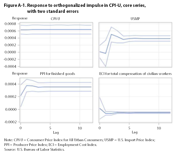
Granger-causality tests using core price indexes (i.e., indexes that exclude food and energy) provide no support for the hypothesis that changes in the ECI have a predictive impact on changes in the CPI or the PPI for finished goods. The reverse proposition—that changes in the CPI and the PPI for finished goods Granger-cause changes in the ECI—also does not hold. An examination of the series’ orthogonalized impulse-response functions, however, suggests that an impulse to the CPI has a significant, long-run impact on the PPI and the ECI, although the effect on the ECI is negative.
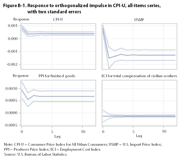
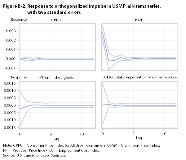
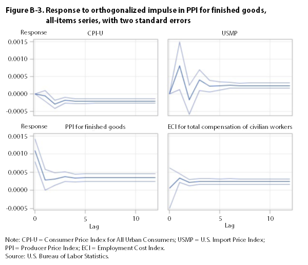
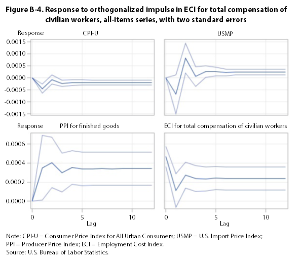
Granger-causality tests using indexes that include food and energy support the hypothesis that the ECI has a predictive impact on the CPI and the PPI for finished goods. These tests also support the hypothesis that the CPI and the PPI for finished goods have a predictive impact on the ECI. An examination of the series’ orthogonalized impulse-response functions indicates that a one-standard-deviation perturbation in the CPI and the PPI for finished goods leads to a significant change in the ECI. Similarly, a one-standard-deviation perturbation in the ECI leads to a significant change in the CPI and the PPI for finished goods. These results may be unduly affected by the worldwide downturn in energy prices that began in 2014.
In sum, tests using core price indexes support the hypothesis that consumer prices affect labor compensation costs, whereas tests using indexes that include food and energy provide no conclusive evidence on the direction of causality.
The U.S. Federal Reserve Board (Fed) policy of “quantitative easing” (QE), or asset-purchase program, has been extensively debated among economists since the economy began to emerge from the financial crisis of 2007–09. QE aimed to provide additional liquidity to credit markets by expanding and diversifying the Fed’s purchase of assets beyond the class of short-term government bonds associated with traditional monetary expansion. The goal was to ease credit markets by lowering the spread on longer term and riskier assets. As former Fed Chairman Ben Bernanke explained, “the Federal Reserve’s credit easing approach focuses on the mix of loans and securities that it holds and on how this composition of assets affects credit conditions for households and businesses.”3
There has been a concern, however, that an expansion of the Fed’s balance sheet could potentially lead to higher inflation. Inflation is a consistent increase, over a period of time, in an economy’s “price level,” a concept referring to the price component of total expenditures on goods and services. Intuitively, one can think of the price level as a CPI index, with the CPI index representing the price of a market basket of goods and services. In reality, the CPI program surveys about 23,000 retail establishments and 6,000 housing units, in 87 urban areas in the United States, to collect prices for approximately 80,000 goods and services. These prices are aggregated into lower and upper level indexes that measure consumer inflation across many sectors of the economy. The broadest measure of consumer inflation is the U.S. city-average, all-items CPI for All Urban Consumers (CPI-U). This index can be interpreted as the price that a representative, or composite, urban consumer pays for a market basket consisting of all consumer goods and services for which the CPI program collects prices.
Concerns about inflation stem, in part, from a basic understanding of monetary expansion in a fractional-reserve banking system. Increases in the money supply can occur when the Fed engages in traditional open-market operations or, in the case of QE, further expands its balance sheet to include longer term and riskier assets. However, this increase in liquidity may not cause inflation if credit markets remain tight (i.e., if the velocity of money declines). When credit markets are tight—e.g., because higher required-reserve levels are enforced, because banks are reluctant to lend and instead “hoard” cash assets, or because money demand rises as interest rates approach zero and returns from investment decline—economic activity will remain constrained and there will be little upward pressure on prices. In other words, for inflation to occur, monetary expansion—by way of traditional short-term government bond purchases or by way of QE-driven purchases of longer term and more diversified asset classes—must result in an increase in aggregate demand.
The role of aggregate demand can be seen in two alternative explanations of how inflation may occur: a “demand-pull” explanation and a “cost-push” explanation. The former suggests that increases in the price level of the economy result from increases in aggregate demand precipitated by traditional Fed monetary expansion. As the Fed funds rate approaches zero and spread volatility increases in a time of economic crisis, QE extends this policy to longer term and riskier assets, thereby aiming to reduce and stabilize the spread of such assets over the Fed funds rate. As loan expansion and risky asset purchases work their way through the economy, business activity expands, firms hire additional workers, and the unemployment rate falls below its “natural,” or equilibrium, rate. Aggregate demand increases, firms boost production, the supply of available workers falls, and firms raise wages in order to attract and retain workers. Aggregate supply increases in the short run, as more workers produce more output, and then falls back to its long-run equilibrium, as costs continue to rise and firms raise prices in response to increased demand.
The second, cost-push explanation of inflation suggests that advances in the economy’s price level may result from cost pressures precipitated by sudden increases in the price of labor or other inputs. In such cases, firms may incur higher input prices and reduce purchases of materials and capital or they may face higher compensation costs and lay off workers. The result is a reduction in aggregate supply, which increases the price level as output falls and goods become scarcer. Moreover, some of the increased costs for materials and labor may be passed on to consumers in the form of higher prices, contributing to a further rise in the price level. If the Fed reacts to a fall in aggregate supply by engaging in open market operations, aggregate demand may increase and firms may continue to raise prices. If the cycle of cost pressures and aggregate-demand increases continues, the result is a consistent increase in prices, known as “cost-push” inflation.
In short, inflation is a series of increases in the price level of the economy. Increases in aggregate demand may “pull up” the price level while costs rise and firms expand production. Alternatively, increases in costs may “push up” the price level as aggregate supply falls, firms reduce production, the Fed embarks on an expansionary monetary policy, or some other set of factors causes aggregate demand to rise after the drop in supply.
From this paradigm arises the question addressed in this article, namely, whether growth in labor compensation costs (a major component of the cost of production) is a predictive indicator of price inflation in components of final demand (cost-push inflation) or whether price inflation in components of final demand (i.e., consumer prices and finished-goods prices) is a predictive indicator of growth in labor compensation costs (demand-pull inflation). In the cost-push scenario, it is expected that the ECI, a measure of compensation growth, will have a predictive impact on the CPI and the PPI for finished goods. In the demand-pull scenario, it is expected that the CPI and the PPI for finished goods will have a predictive impact on the ECI. These relationships are expected to hold after controlling for input prices (as measured by the PPI indexes for crude and intermediate goods), import prices (as measured by the USMP), demand shocks (as measured by output and unemployment gaps), and, in one variation of the model, productivity.
One immediate implication of this discussion is that the direction of price transmission can be ambiguous. In the cost-push scenario, inflation begins with upward pressure on labor compensation costs and input prices, leading one to expect that an increase in the ECI would occur before an increase in the CPI or the PPI for finished goods. In the demand-pull scenario, inflation begins with aggregate-demand increases that motivate firms to hire more workers, leading one to expect that increases in the CPI and the PPI for finished goods would occur before an increase in the ECI. In either case, labor costs are an important part of the story.4
Economic theory posits that labor costs, a component of the marginal cost of production, are a determining factor in the level of prices and that increases in labor costs can lead to higher consumer prices. The argument is articulated by Richard Layard, Stephen Nickell, and Richard Jackman:
…when buoyant demand reduces unemployment (at least relative to recent experienced levels), inflationary pressure develops. Firms start bidding against each other for labour, and workers feel more confident in pressing wage claims. If the inflationary pressure is too great, inflation starts spiraling upwards: higher wages lead to higher price rises, leading to still higher wage rises, and so on. This is the wage-price spiral.5
However, much of the empirical literature finds that wage inflation does not predict price inflation.6 The cost-push scenario may be inoperative if productivity increases. When the productivity of workers increases, firms can reduce prices on each unit of output (all else equal). If wages rise at the same rate as productivity, firms “break even” and do not incur higher costs as production expands and wages rise.7 Moreover, the extent of price transmission depends on a variety of economic factors, such as the relative negotiating power of buyers and sellers, the elasticity of demand and supply, the extent of price competition among producers, the costs of different inputs to production, and the interplay between cyclical and structural fluctuations in the labor market. As noted by Fed Chairwoman Janet Yellen, it has been shown that, historically, slack in the labor market “has accounted for only a small portion of the fluctuations in inflation.”8 Moreover, the timing and extent of the impact of wage pressures on prices are difficult to pin down.9
However, the literature does provide support for the reverse proposition, namely, that price inflation can signal wage inflation.10 As already noted, this effect can occur under a demand-pull scenario in which unemployment declines lead to aggregate-demand and price-level increases, followed by increases in labor compensation costs. Here, the cost-push scenario is inoperative, even though unemployment declines tighten the labor market and generate upward pressure on labor compensation costs.
Despite these findings and notwithstanding recent declines in labor market slack, inflation concerns continue to be expressed. Are they warranted? To address this question, this article tests the propositions (1) that wage inflation precedes price inflation and (2) that price inflation precedes wage inflation. A VECM is developed to test if one of these propositions holds, or if both hold (in which case no definitive conclusion can be drawn). The model uses ECI, PPI, USMP, and CPI data for the period from the first quarter of 2001 to the fourth quarter of 2015. Tests on the core series (i.e., indexes that include all items less food and energy) provide some support for the demand-pull hypothesis, whereas tests on the all-items series are inconclusive. The next section provides an overview of the U.S. Bureau of Labor Statistics (BLS) price-index programs and the data used in this article. The section on methodology and results follows.
The Consumer Price Index (CPI), the Producer Price Index (PPI), the U.S. Import Price Index (USMP), and the Employment Cost Index (ECI)—all published regularly by BLS—are designated as Principal Federal Economic Indicators by the Office of Management and Budget. All four measures provide information on price change and are used as a guide in detecting and responding to inflationary pressures in the economy and for such purposes as deflating economic series and adjusting price agreements. Their users include the U.S. President, Congress, the Fed, academics, private citizens, and decisionmakers in business, government, and labor.
Although each index measures price change, it does so from a different perspective. The CPI measures the average change over time in the prices paid by urban consumers for a market basket of goods and services. The CPI is thus a measure of price change from the perspective of an urban consumer. The PPI measures the average change over time in the selling prices received by producers of goods and services.11 The PPI is thus a measure of price change from the perspective of the producer. The ECI measures “the change in the cost of labor, independent of the influence of employment shifts among occupations and industry categories.”12 The ECI is thus “an indicator of cost pressures within companies that could lead to price inflation for finished goods and services.”13 The USMP measures the average change over time in imported goods; it is thus a measure of price change from the perspective of either consumers or producers who purchase imported goods.14
By adopting a different measurement perspective, each index captures price change at a different stage in the value chain encompassing the production and sale of goods and services. The ECI picks up changes in compensation paid to employees. The USMP picks up changes either (1) in the prices of imported final goods purchased by consumers or businesses or (2) in the prices of imported goods purchased by firms as inputs to production. The PPI picks up changes in the prices received by producers of goods and services, which include inputs used at different stages of production and final goods purchased by final-demand consumers (including government and business).15 Finally, the CPI picks up changes in the prices paid by urban consumers. Because of their unique characteristics, the four broad measures of price change allow for the development of economic models for examining price transmission across different stages of the value chain.
The analysis presented in the next section relies primarily on core index series—i.e., indexes that exclude food and energy—in order to focus on underlying trends; however, analysis based on indexes that include food and energy is also presented. The specific index series used are the core versions of the U.S. city-average, all-items CPI for All Urban Consumers (CPI-U); the PPI for finished goods; the PPI for crude goods (crude materials) and intermediate goods (intermediate materials, supplies, and components); the USMP for all commodities; and the ECI for total compensation of all civilian workers. No further breakdowns of these high-level aggregate indexes are used.
The CPI-U and the PPI for finished goods serve as measures of changes in final-demand prices. The PPI indexes for crude and intermediate goods serve as supply-shock control variables that measure changes in the cost of inputs at the crude and intermediate stages of production. The USMP serves as a supply-shock measure of changes in import prices. Finally, the ECI is used as a measure of changes in labor compensation costs. All of these series tend to move together and to trend upward over time. (See
The purpose of this article is to empirically test the proposition that not only do the series move together, but a change in the movement of one series (in particular, the ECI) has a systematic impact on changes in the movement of other series (in particular, the CPI and the PPI for finished goods). This is done with a vector error-correction model (VECM), explained in the next section. The number of observations is constrained by ECI’s historical coverage, which begins in the first quarter of 2001. Thus, the data series run from the first quarter of 2001 to the final quarter of 2015 (the most recent quarter for which data were available at the time the analysis was conducted). The ECI data are collected every 3 months and published quarterly. As stated in the BLS Handbook of Methods, ECI data collection is conducted as follows: “Although initial data collection occurs at any time of the year, ECI and ECEC updates are conducted over a 6-week timeframe for the pay period that includes the 12th day of the month for the months of March, June, September, and December [emphasis added].”16 To maintain data consistency, the analysis uses CPI, PPI, and USMP data for March, June, September, and December.17
In January 2014, the PPI program switched to the Final Demand–Intermediate Demand price-index aggregation structure, which was “the culmination of a long-standing PPI objective to improve the current SOP [Stage of Processing] aggregation system by incorporating PPIs for services, construction, government purchases, and exports.”18 Unfortunately, high-level indexes under the new aggregation structure do not provide sufficient history for the analysis in this article.19 Therefore, the article uses PPI index series under the old, SOP aggregation structure (i.e., PPIs for finished goods and for crude and intermediate goods). These series go back to 2001, providing sufficient coverage parallel to that for the ECI, the USMP, and the CPI.
In addition to including price indexes, the model employed in the analysis controls for demand shocks and productivity. Demand-shock variables are the output gap and the unemployment gap. The output gap is defined as the difference between real gross domestic product (GDP) and potential real GDP.20 The unemployment gap is defined as the difference between the observed unemployment rate and the natural rate of unemployment.21 The control variable for labor productivity is based on quarterly data from BLS.22
This section develops a vector autoregression (VAR) model to examine (1) the extent to which changes in labor compensation costs drive subsequent price increases and (2) the extent to which consumer and finished-goods prices drive subsequent compensation-cost increases. A VAR model estimates a system of equations in which each value of a time series is expressed as a linear combination of itself, the values of other time series, and lagged values of those series. Here, a VAR model is estimated for four core series: the U.S. city-average, all-items CPI-U (less food and energy); the USMP (excluding fuels); the PPI for finished goods (less food and energy); and the ECI for total compensation of civilian workers. In addition, the core PPI series for crude and intermediate goods are used as control variables, as are measures of the output and unemployment gaps. The analysis employs seasonally adjusted series, taking their natural logarithms.23 Working with logarithms is beneficial because it allows multiplicative relations to be expressed in additive terms and because it converts exponential growth to linear growth. These advantages allow the use of linear models.
In estimating a time-series model, one should ensure that the data are stationary, i.e., that the means, variances, and covariances of the time series exist and are independent of time. If the series are nonstationary, or integrated, standard tests for the significance of the estimated coefficients will be invalid and may yield support for potentially spurious relations. For this article, a battery of unit-root tests, including the augmented Dickey–Fuller test and the Phillips–Peron test, were performed to check for stationarity. These tests, together with an examination of autocorrelation functions, indicated that the series, expressed in log terms, were nonstationary. The series were then converted to percentage-growth form by taking the first differences of each logged series—a standard transformation that often induces stationarity. After this transformation, the battery of stationarity tests was repeated, indicating that the series are stationary in the percentage-growth form.
To determine the correct lag structure of the VAR, two approaches were employed. First, partial autocorrelation functions (PACFs) were examined in order to observe the potential order of any existing autoregressive (AR) process. A PACF plots the partial autocorrelation between a variable and its own values lagged n times. This partial autocorrelation is defined as the correlation between the variable and its nth lag, conditional on the set of lagged values between time t and time t − n (e.g., the correlation between values two periods apart is conditional on the value in the intermediate period). Examining PACFs is theoretically helpful because, in an AR model, the PACF should fall to zero past the order of the model. In other words, a first-order AR model, known as AR(1), should have one nonzero partial autocorrelation. Second, a procedure was implemented to determine which lag structure would minimize the corrected Akaike information criterion (AICC) and Schwarz (Bayesian) information criterion (BIC). These criteria provide justification for model selection when one faces a tradeoff between goodness of fit and parsimony.
The examination of PACFs indicated that it was essential to include one lag of each variable, with the second lag being marginal. The AICC and BIC were both minimized by an AR(1) model, so that specification was used. The final VAR model also included constant and trend terms, as well as a dummy variable that corrects for an exogenous structural break in the data. That break occurs around the fourth quarter of 2008. In particular, the rate of growth in the ECI suddenly decreases, resulting in a less steep upward trend. The other series are characterized by a significant, one-period decline at the same point. This break in trend could be a reflection of the 2007−09 financial crisis exerting a moderating influence on inflationary trends.
In modeling time series, one should also consider whether the series are cointegrated (i.e., whether they share a common stochastic trend). When series are cointegrated, they individually appear to be nonstationary, although, in fact, certain linear combinations of them are stationary. To test for the presence of cointegration in the series, the Johansen cointegration rank test was employed. Because it has been shown that the Johansen tests are inaccurate in the presence of dummies for structural change, the VAR model was estimated without these dummies for the purpose of determining the number of cointegrating vectors. This procedure indicated that the system is characterized by three cointegrating vectors. To account for this cointegration, a VECM was estimated. The VECM is a restricted VAR model whose specification is altered to account for the nonstationarity of the cointegrated series. The VECM restricts the long-run behavior of the endogenous variables so that they converge to the cointegrating relationships without interfering with the short-run dynamics. The final model can be expressed as follows:
![]() ,
,
where Xt = (CPI-U, PPI for finished goods, USMP, ECI for total compensation of civilian workers); µ0 is the constant; φ and γ' are the “5 × 3” matrices of the loading coefficients and cointegrating vectors, respectively (under the assumption of three cointegrating vectors); Γi is the gamma function; β1 and β2 are the estimated coefficients; Dt is the vector of the dummy variables representing the structural break and the linear trend; Pt is the vector of the control variables for input prices, the unemployment gap, and the output gap; and εt is the residual.24
This VECM specification was used to test for Granger causality between the series. A variable is said to Granger-cause another variable if adding lagged values of the former to an autoregressive model of the latter improves the predictive power of the model. A Wald test was conducted on the null hypothesis that there was no Granger causality between the series. Wald tests yield a statistic that allows the examination of the hypothesis that the value of a parameter estimated from a certain sample is the true value of that parameter. In the case of Granger causality, Wald tests indicate whether or not future values of one series can be predicted on the basis of past values of one or more other series.
Wald tests performed for this article reject the null hypotheses (1) that the ECI does not Granger-cause the USMP and (2) that the USMP does not Granger-cause the PPI and the ECI. (See table 1.) In all other instances, the tests fail to reject the null hypothesis of no Granger causality. Thus, with respect to
| Variable | Wald statistic | p-value |
|---|---|---|
| Independent variable: CPI | ||
| USMP | 0.10 | 0.7492 |
| PPI | 1.19 | .2763 |
| ECI | .02 | .8928 |
| Model | 7.34 | .3942 |
| Independent variable: USMP | ||
| CPI | .02 | .8850 |
| PPI | 2.61 | .1061 |
| ECI | 4.62 | .0317 |
| Model | 12.02 | .1000 |
| Independent variable: PPI | ||
| CPI | 1.64 | .1998 |
| USMP | .66 | .4158 |
| ECI | .01 | .9064 |
| Model | 3.25 | .8605 |
| Independent variable: ECI | ||
| CPI | .21 | .6472 |
| USMP | 4.41 | .0357 |
| PPI | 1.80 | .1802 |
| Model | 16.37 | .0219 |
Note: CPI = Consumer Price Index; USMP = U.S. Import Price Index; PPI = Producer Price Index; ECI = Employment Cost Index. Source: U.S. Bureau of Labor Statistics. | ||
Given the complex nature of the VECM, it is difficult to interpret the modeled coefficients. For this reason, impulse-response functions were used to provide insight into the VECM. Impulse-response functions show the impact of an exogenous one-standard-deviation shock to one series on the current and future values of all other series. (Shocks to one series often occur simultaneously with similar shocks to other series.) To examine the unique effect of each exogenous shock, the model’s residuals were orthogonalized. This process used a Cholesky decomposition in which the covariance matrix is expressed as the product of a lower triangular matrix and its conjugate transpose. The decomposition ensures that a shock to any one variable will only affect variables ordered after that variable in the VECM. Although many contemporary macroeconomists use specific structural restrictions to test their hypotheses, the present analysis was limited to determining the high-level relationships between the series.
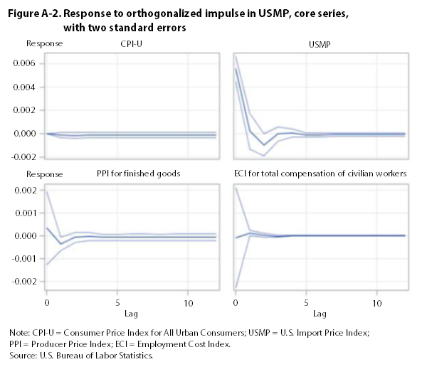
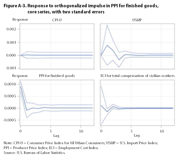
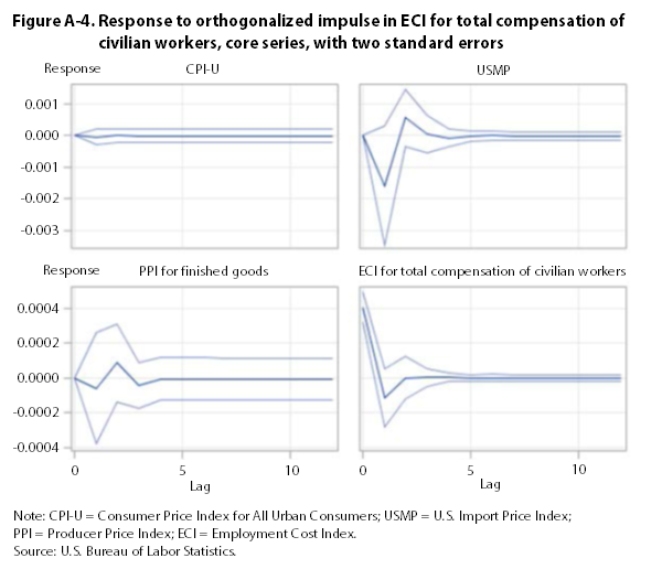
Once the residuals were orthogonalized, impulse-response functions were constructed from the VECM coefficients. These functions—represented in diagrams—show the response of each series to an exogenous change in other series. All impulse response functions are calculated with 95-percent confidence bands. When both of these bands are above or below the zero line, one could say that there is a 95-percent likelihood that a response is significantly different from zero.
The impulse-response functions presented in appendix A show that a one-standard-deviation perturbation in the CPI leads to a significant increase in the PPI and the USMP. It also leads to a decrease in the ECI. The impulse responses for the USMP, the PPI, and the ECI are not significantly different from zero. Thus, over the period examined, changes in the CPI are followed by changes in the PPI, the USMP, and the ECI. This result lends some support to the demand-pull hypothesis, according to which increases in aggregate demand can “pull up” the price level, but only with respect to finished-goods prices, because the ECI falls in response to a positive shock to the CPI. However, the results do not provide support for the reverse, cost-push hypothesis, according to which increases in compensation costs are followed by increases in consumer or finished-goods prices.
The same battery of tests were conducted with the use of “all-items” indexes—i.e., CPI and PPI indexes including food and energy—and the USMP including fuels. (See table 2.) The Wald tests for Granger causality run on the VECM for these indexes reject the null hypothesis that the ECI does not Granger-cause the CPI, the PPI, and the USMP. The tests also reject the null hypotheses (1) that the PPI does not Granger-cause the USMP and the ECI, (2) that the CPI does not Granger-cause the ECI (at the 10-percent significance level), and (3) that the USMP does not Granger-cause the CPI and the ECI. Therefore, tests based on indexes that include food and energy support the cost-push hypothesis (that changes in the ECI are followed by changes in the CPI and the PPI) and the demand-pull hypothesis (that changes in the PPI and the CPI are followed by changes in the ECI).25
| Variable | Wald statistic | p-value |
|---|---|---|
| Independent variable: CPI | ||
| USMP | 19.66 | <.0001 |
| PPI | 2.09 | .1478 |
| ECI | 2.98 | .0843 |
| Model | 31.66 | <.0001 |
| Independent variable: USMP | ||
| CPI | 10.77 | .0010 |
| PPI | 1.45 | .2291 |
| ECI | 5.32 | .0211 |
| Model | 25.11 | .0007 |
| Independent variable: PPI | ||
| CPI | 1.96 | .1617 |
| USMP | 6.42 | .0113 |
| ECI | 4.12 | .0423 |
| Model | 22.58 | .0006 |
| Independent variable: ECI | ||
| CPI | 5.14 | .0234 |
| USMP | 4.45 | .0349 |
| PPI | 5.59 | .0181 |
| Model | 16.56 | .0204 |
Note: CPI = Consumer Price Index; USMP = U.S. Import Price Index; PPI = Producer Price Index; ECI = Employment Cost Index. Source: U.S. Bureau of Labor Statistics. | ||
The impulse-response functions for the all-items series show that a one-standard-deviation perturbation in the ECI, the PPI, and the CPI has a significant, long-run impact on all of the other all-items series. (See appendix B.) A similar impulse in the USMP has no discernible long-run effect on other all-items series.26
Additional model specifications were constructed to assess the robustness of the results. For example, one specification included an estimate of productivity in the VECM. This specification did not noticeably alter the results obtained from the model. Another specification used unit labor costs in place of the ECI. This specification behaved similarly to the first, although with much increased volatility. Further alternative specifications used quarterly average data (for the CPI, the PPI, and the USMP) instead of end-of-quarter observations. These specifications did not significantly change the results.
In response to the 2007–09 financial crisis, the Fed embarked on a policy of quantitative easing, which resulted in an unprecedented increase in the Fed’s balance sheet. This increase raised concerns about possible long-term inflationary effects. There are two hypotheses about the causes of potential inflation: a demand-pull hypothesis, which suggests that inflation results from increases in aggregate demand, and a cost-push hypothesis, which posits that inflation stems from increases in labor compensation costs.
Using core indexes that exclude food and energy, this article finds no support for the cost-push hypothesis—a result in line with much of the empirical literature on wage–price inflation. Granger-causality tests fail to reject the null hypotheses (1) that the ECI does not Granger-cause the CPI and the PPI and (2) that the CPI and the PPI do not Granger-cause the ECI. Impulse-response functions, however, show that changes in the CPI are followed by changes in the ECI, the PPI, and the USMP, although the effect on the ECI is negative. These results lend support to the demand-pull hypothesis.
Using indexes that include food and energy, Granger-causality tests reject the null hypothesis that the ECI does not Granger-cause the CPI, the PPI, and the USMP. They also reject the null hypothesis that the CPI and the PPI do not Granger-cause the ECI. Orthogonalized impulse-response functions indicate that a one-standard-deviation perturbation in the ECI, the PPI, and the CPI has a significant, long-run impact on all other all-items series. Thus, tests employing indexes that include food and energy are inconclusive on the direction of causality. This result may be due to the downturn in energy prices that occurred toward the end of the study period.
In sum, tests using core series lend support to the demand-pull hypothesis, whereas tests using series that include food and energy are inconclusive.
Akaike, Hirotugu. “A new look at the statistical model identification.” IEEE Transactions on Automatic Control, vol. 19, no. 6 (December 1974), pp. 716–723.
Commandant Benoit. “Note sur une méthode de résolution des équations normales provenant de l'application de la méthode des moindres carrés à un système d'équations linéaires en nombre inférieur à celui des inconnues (Procédé du Commandant Cholesky).” Bulletin Géodésique, vol. 2 (1924), pp. 67–77.
Dickey, David A., and Wayne A. Fuller. “Distribution of the estimators for autoregressive time series with a unit root.” Journal of the American Statistical Association, vol. 74, no. 366 (1979), pp. 427–431.
Ghali, Khalifa. “Wage growth and the inflation process: a multivariate cointegration analysis.” Journal of Money, Credit, and Banking, vol. 31, no. 3 (August 1999), pp. 417–431.
Gordon, Robert J. “The role of wages in the inflation process.” American Economic Review Papers and Proceedings, vol. 78, no. 2 (May 1988), pp. 276–283.
Granger, Clive W. J. “Investigating causal relations by econometric models and cross-spectral methods.” Econometrica, vol. 37, no. 3 (August 1969), pp. 424–438, http://www.sonoma.edu/users/c/cuellar/econ411/Granger.pdf.
———. “Time series analysis, cointegration, and applications.” American Economic Review, vol. 94, no. 3 (2004), pp. 421–425, https://www.nobelprize.org/prizes/economic-sciences/2003/granger/lecture/.
Hamilton, James D. Time series analysis, vol. 2. Princeton, NJ: Princeton University Press, 1994.
Hess, Gregory D., and Mark E. Schweitzer. “Does wage inflation cause price inflation?” Federal Reserve Bank of Cleveland, Policy Discussion Papers (April 2000), p. 9, https://papers.ssrn.com/sol3/papers.cfm?abstract_id=1025464.
Hurvich, Clifford M., and Chih-Ling Tsai. “Regression and time series model selection in small samples.” Biometrika, vol. 76 (1989), pp. 297–307.
Johansen, Søren. “Estimation and hypothesis testing of cointegration vectors in Gaussian vector autoregressive models.” Econometrica, vol. 59, no. 6 (1991), pp. 1551–1580.
Jonsson, Magnus, and Stefan Palmqvist. “Do higher wages cause inflation?” Working Paper no. 159. Stockholm, Sweden: Sveriges Riksbank, April 2004, p. 2, http://www.riksbank.se/Upload/WorkingPapers/WP_159.pdf.
Kennedy, Peter. A guide to econometrics. Cambridge, MA: The MIT Press, 2003.
Knotek II, Edward S., and Saeed Zaman. “On the relationships between wages, prices, and economic activity.” Federal Reserve Bank of Cleveland, Inflation Central (August 19, 2014), https://www.clevelandfed.org/newsroom-and-events/publications/economic-commentary/2014-economic-commentaries/ec-201414-on-the-relationships-between-wages-prices-and-economic-activity.aspx.
Layard, Richard, Stephen Nickell, and Richard Jackman. The unemployment crisis. Oxford, UK: Oxford University Press, 1994.
Hu, Luojia, and Maude Toussaint-Comeau. “Do labor market activities help predict inflation?” Federal Reserve Bank of Chicago, Economic Perspectives, vol. 34, no. 2 (2nd quarter 2010), p. 52, https://www.chicagofed.org/digital_assets/publications/economic_perspectives/2010/2qtr2010_part2_hu_toussaint_comeau.pdf.
Mehra, Yash P. “Unit labor costs and the price level.” Federal Reserve Bank of Richmond, Economic Review, vol. 79, no. 4 (Fall 1993), pp. 35–52, http://richmondfed.org/publications/research/economic_quarterly/1993/fall/pdf/mehra.pdf.
Phillips, Peter C. B., and Pierre Perron. “Testing for a unit root in time series regression.” Biometrika, vol. 75, no. 2 (1988), pp. 335–346.
Rissman, Ellen R. “Sectoral wage growth and inflation.” Federal Reserve Bank of Chicago, Economic Perspectives (July/August 1995), pp. 16–28, https://www.chicagofed.org/publications/economic-perspectives/1995/07julaug1995-part2-rissman.
Schwarz, Gideon E. “Estimating the dimension of a model.” Annals of Statistics, vol. 6, no. 2 (1978), pp. 461–464.
Sims, Christopher A. “Money, income, and causality.” The American Economic Review, vol. 62, no. 4 (1972), pp. 540–552, http://www.sonoma.edu/users/c/cuellar/econ411/Sims.pdf.
———. “Macroeconomics and reality.” Econometrica, vol. 48, no. 1 (1980), pp. 1–48, http://www.pauldeng.com/pdf/Sims%20macroeconomics%20and%20reality.pdf.
———. “Are forecasting models usable for policy analysis?” Federal Reserve Bank of Minneapolis, Quarterly Review, vol. 10, no. 1 (1986), pp. 2–16, http://www.minneapolisfed.org/research/QR/QR1011.pdf.
Swanson, Norman R., and Clive W. Granger. “Impulse response functions based on a causal approach to residual orthogonalization in vector autoregressions.” Journal of the American Statistical Association, vol. 92, no. 437 (1997), pp. 357–367.
Wald, Abraham. “Tests of statistical hypotheses concerning several parameters when the number of observations is large.” Transactions of the American Mathematical Society, vol. 54, no. 3 (1943), pp.
Weinhagen, Jonathan C. “An empirical analysis of price transmission by stage of processing.” Monthly Labor Review (November 2002), https://www.bls.gov/opub/mlr/2002/11/art1full.pdf.
———. “Price transmission within the PPI for intermediate goods.” Monthly Labor Review (May 2005), https://www.bls.gov/opub/mlr/2005/05/art4full.pdf.
———. “Price transmission: from crude petroleum to plastics products.” Monthly Labor Review (December 2006), https://www.bls.gov/opub/mlr/2006/12/art4full.pdf.
———. “Price transmission effects through three stages of food production.” Monthly Labor Review (December 2012), https://www.bls.gov/opub/mlr/2012/12/art2full.pdf.
Wen, Yi, and Maria A. Arias. “What does money velocity tell us about low inflation in the U.S.?” Federal Reserve Bank of St. Louis (September 1, 2014).
ACKNOWLEDGMENT: The authors would like to thank Peter Zadrozny, Kenneth Stewart, John Layng, and David Friedman for providing helpful commentary in the drafting of this article.
Jonathan D. Church and Bradley Akin, "Examining price transmission across labor compensation costs, consumer prices, and finished-goods prices," Monthly Labor Review, U.S. Bureau of Labor Statistics, April 2017, https://doi.org/10.21916/mlr.2017.13
1 The U.S. Import Price Index, referred to as USMP in this article, is produced by the U.S. Bureau of Labor Statistics International Price Program.
2 The preliminary draft of this article was completed in early 2016 and used PPI indexes published under the old, Stage of Processing (SOP) aggregation system. Subsequently, “effective with the January 2016 PPI data release in February 2016, PPI ceased the calculation and publication of the SOP versions of these indexes. Going forward, data users wishing to track prices for finished goods, processed goods for intermediate demand (intermediate goods), unprocessed goods for intermediate demand (crude goods), or any of the former SOP-based component indexes will need to utilize the corresponding index codes from the FD–ID aggregation system.” See “PPI Stage of Processing duplicate codes discontinued,” Producer Price Indexes (U.S. Bureau of Labor Statistics), https://www.bls.gov/ppi/sopseriesids.htm. Corresponding index codes can be found at https://www.bls.gov/ppi/fdidconcordance.htm.
3 Ben S. Bernanke, “The crisis and the policy response” (Stamp lecture, London School of Economics, London, England, January 13, 2009), http://www.federalreserve.gov/newsevents/speech/bernanke20090113a.htm.
4 Luojia Hu and Maude Toussaint-Comeau summarize the idea as follows: “It is unclear whether wage inflation causes price inflation or vice versa. If rising demand for goods and services reduces unemployment (causing it to fall below some natural rate), inflationary pressures might develop as firms bid against each other for labor and as workers feel more confident in pressing for higher wages. Then higher wages could lead to still higher prices. (In an extreme case, this might lead to a wage–price spiral, which we saw in the United States during the 1970s [Perry, 1978]). However, if rising demand for goods and services (for example, too much money chasing too few goods) induces firms to raise their prices, these price increases and greater profits could entice workers to demand higher wages. In such an environment, inflation could lead to wage growth (Friedman, 1956; Cagan, 1972; and Barth and Bennett, 1975).” See Hu and Toussaint-Comeau, “Do labor market activities help predict inflation?” Economic Perspectives, vol. 34, no. 2 (Federal Reserve Bank of Chicago, 2nd quarter 2010), p. 52, https://www.chicagofed.org/digital_assets/publications/economic_perspectives/2010/2qtr2010_part2_hu_toussaint_comeau.pdf.
5 Richard Layard, Stephen Nickell, and Richard Jackman, The unemployment crisis (Oxford, UK: Oxford University Press, 1994), p. 11, quoted in Magnus Jonsson and Stefan Palmqvist, “Do higher wages cause inflation?” Working Paper no. 159 (Stockholm, Sweden: Sveriges Riksbank, April 2004), p. 2, http://www.riksbank.se/Upload/WorkingPapers/WP_159.pdf; and Gregory D. Hess and Mark E. Schweitzer, “Does wage inflation cause price inflation?” Policy Discussion Papers (Federal Reserve Bank of Cleveland, April 2000), p. 1, https://fraser.stlouisfed.org/scribd/?item_id=495634&filepath=/files/docs/historical/frbclev/pdp/frbclv_pdp_200004_010.pdf&start_page=1.
6 See, for example, Hess and Schweitzer, “Does wage inflation cause price inflation?”; Hu and Toussaint-Comeau, “Do labor market activities help predict inflation?”; Yash P. Mehra, “Unit labor costs and the price level,” Economic Review, vol. 79, no. 4 (Federal Reserve Bank of Richmond, Fall 1993), http://richmondfed.org/publications/research/economic_quarterly/1993/fall/pdf/mehra.pdf; and Ellen R. Rissman, “Sectoral wage growth and inflation,” Economic Perspectives (Federal Reserve Bank of Chicago, July/August 1995), https://www.chicagofed.org/publications/economic-perspectives/1995/07julaug1995-part2-rissman.
7 A simple equation makes this point clear: W = P × MP = MRP, where W = wages, P = price, MP = marginal product, and MRP = marginal revenue product. In other words, the wage level (i.e., compensation) is equal to the price of output (P) multiplied by the incremental quantity of output produced by a worker (MP), and price times quantity equals revenue (MRP). If productivity (MP) rises at the same rate as wages (W), price (P) remains unchanged and W = MRP. As noted by Hu and Toussaint-Comeau, “If productivity growth drives higher wages, the firm does not have to pass on higher wages into higher prices. Increased productivity therefore should curb inflationary pressures.” See Hu and Toussaint-Comeau, “Do labor market activities help predict inflation?” p. 52.
8 Janet L. Yellen, “Labor market dynamics and monetary policy” (speech, Federal Reserve Bank of Kansas City Economic Symposium, Jackson Hole, WY, August 22, 2014), https://www.federalreserve.gov/newsevents/speech/yellen20140822a.htm.
9 Ibid.
10 See, for example, Hess and Schweitzer, “Does wage inflation cause price inflation?”; Hu and Toussaint-Comeau, “Do labor market activities help predict inflation?”; Mehra, “Unit labor costs and the price level”; and Rissman, “Sectoral wage growth and inflation.”
11 “Frequently asked questions,” Producer Price Indexes (U.S. Bureau of Labor Statistics), http://stats.bls.gov/ppi/ppifaq.htm#1.
12 Handbook of methods, chapter 8, “National compensation measures” (U.S. Bureau of Labor Statistics), https://www.bls.gov/opub/hom/pdf/homch8.pdf.
13 John W. Ruser, “The Employment Cost Index: what is it?” Monthly Labor Review, September 2001, p. 3, https://www.bls.gov/opub/mlr/2001/09/art1full.pdf.
14 Handbook of methods, chapter 15, “International price indexes,” https://www.bls.gov/opub/hom/pdf/homch15.pdf.
15 This article uses PPIs for finished goods based on the old, SOP aggregation system. However, price indexes based on the new, FD–ID system pick up both final goods and final services purchased by final-demand consumers.
16 Handbook of methods, chapter 8, p. 4.
17 The analysis is also conducted with the use of quarterly averages of the CPI, the PPI, and the USMP.
18 “Producer Price Index transitions from the Stage-of-Processing to the Final Demand–Intermediate Demand aggregation system,” Producer Price Indexes (U.S. Bureau of Labor Statistics), https://www.bls.gov/ppi/fdidtransition.htm.
19 The PPI website (see ibid.) states that “nearly all new FD–ID goods, services, and construction indexes provide historical data back to either November 2009 or April 2010, while the indexes for goods that correspond with the historical SOP indexes go back to the 1970s or earlier.”
20 Real gross domestic product (GDP) data, presented in chained 2009 dollars, are obtained from the U.S. Bureau of Economic Analysis, https://www.bea.gov/national/index.htm#gdp. Potential real GDP data, also presented in chained 2009 dollars, are produced by the Congressional Budget Office and obtained from FRED, Federal Reserve Bank of St. Louis, http://research.stlouisfed.org/fred2/series/GDPPOT.
21 Unemployment data are obtained from the U.S. Bureau of Labor Statistics, https://www.bls.gov/cps/. Data on the natural rate of unemployment (NROU) are produced by the Congressional Budget Office and obtained from FRED, Federal Reserve Bank of St. Louis, http://research.stlouisfed.org/fred2/series/NROU. NROU data are produced quarterly, whereas unemployment data are produced monthly. For a given quarter, the unemployment gap is calculated as the difference between the quarterly average rate of unemployment and the NROU for that quarter.
22 “Labor productivity and costs” (U.S. Bureau of Labor Statistics), https://www.bls.gov/lpc/. This article uses labor productivity data for the nonfarm business sector.
23 USMP series are not seasonally adjusted.
24 For general information about the methodology, see James D. Hamilton, Time series analysis, vol. 2 (Princeton University Press, 1994); and Peter Kennedy, A guide to econometrics (Cambridge, MA: The MIT Press, 2003).
25 This result may reflect CPI changes due to the recent drop in energy prices. These same tests were previously run through the first quarter of 2014, using all-items indexes (i.e., CPI and PPI indexes including food and energy and the USMP including fuels). The tests for these indexes provided support for the cost-push hypothesis, but not for the demand-pull hypothesis. The Wald tests for Granger causality run on the VECM rejected the null hypothesis that the ECI does not Granger-cause the CPI, the PPI, and the USMP. The tests also rejected the null hypotheses (1) that the PPI does not Granger-cause the USMP, (2) that the CPI does not Granger-cause the USMP, and (3) that the USMP does not Granger-cause the CPI and the ECI. The tests did not reject the null hypotheses that the PPI does not Granger-cause the ECI and that the CPI does not Granger-cause the ECI.
26 This result may reflect CPI changes due to the recent drop in energy prices. These tests were previously run through the first quarter of 2014, using all-items series. A one-standard-deviation perturbation in the ECI was found to have no significant long-run impact on any of the other all-items series. A similar perturbation in the USMP had a long-run effect on the all-items CPI and PPI series, whereas a perturbation in the all-items PPI series did not have any discernable impact on the other series.